Submit your Excel / VBA Question
|
Use the adjacent form to submit your Excel / VBA question and have it answered publicly by Excel Savants.
Please note that Excel Savants will not provide code for sophisticated VBA macros using this free channel but will provide the code for simple macros and address specific questions about what VBA arguments to use and why code is not functioning as intended. If you'd like to have Excel Savants code a custom macro, you may submit your request below and you can an expect a private response with a project bid within 1 business day. Visit the Best of Excel & VBA Resources page for links to additional Excel/VBA resources. |
|
Please consider supporting the Excel Savants Answer Forum by visiting our advertisers:
Answer Forum Entries
Conditional Formatting
VBA Programming and Automation
Excel Software & PC
Finance
Conditional Formatting
- Change font size based on data in another cell
- Highlight cells based on data in another cell
- Hide a row using a formula based on a condition
VBA Programming and Automation
- External data import errors
- Splitting a single Excel column of data into two columns using RPA automation
- VBA benefit of using Select Case over If-Then
- VBA to return HEX color code of cell's background color
- VBA code to print range of cells based on a trigger word in another workheet
- VBA argument to move data from one sheet onto another at a specified time
- Updating Excel based planner based on Google calendar entries
Excel Software & PC
- Excel version recommendation
- PC to Mac Excel file compatibility
- Permanently associating workbook file type with preferred version of Excel
- Forgot password for Excel 2010 protected workbook
- Most useful MS Excel trick
- Why are there 16,384 columns in Excel 2016?
Finance
Excel version purchase recommendation
01/22/2022

I am budget conscious and don't currently have Microsoft Office. What version of Excel/Office would you recommend I purchase?
Microsoft did away with perpetual licenses for its Office software in 2018 and moved to (revenue maximizing) subscription based pricing. Office 2019 is the last version of Office you can purchase that still offers a perpetual license. The current version of Microsoft Office is Office 365 which costs $69.99/ yr.
However, in terms of functionality and compatibility there are virtually no differences between Office 365 and Office 2019. Microsoft claims that the advantage of their subscription model is that it's regularly pushing small software updates. This is supposedly more user-friendly than Office 2019 where updates are installed as larger and more infrequent “service packages” which may be disruptive if they are pushing too many user experience changes at once. Personally I think this a very weak value proposition and find the perpetual license much more compelling than the subscription based Office 365. It’s possible to purchase an Office 2019 perpetual license for less than the cost of a 1 yr. subscription to Office 365. Amazon sells the offical retail boxed version of Office 2019 (Professional Plus) for $60.* The Professional Plus version is the most comprehensive version of Office 2019 that Microsoft offered and includes Word, Excel, PowerPoint, OneNote, Outlook, Access, Publisher, OneDrive as well as Skype for Business.
However, in terms of functionality and compatibility there are virtually no differences between Office 365 and Office 2019. Microsoft claims that the advantage of their subscription model is that it's regularly pushing small software updates. This is supposedly more user-friendly than Office 2019 where updates are installed as larger and more infrequent “service packages” which may be disruptive if they are pushing too many user experience changes at once. Personally I think this a very weak value proposition and find the perpetual license much more compelling than the subscription based Office 365. It’s possible to purchase an Office 2019 perpetual license for less than the cost of a 1 yr. subscription to Office 365. Amazon sells the offical retail boxed version of Office 2019 (Professional Plus) for $60.* The Professional Plus version is the most comprehensive version of Office 2019 that Microsoft offered and includes Word, Excel, PowerPoint, OneNote, Outlook, Access, Publisher, OneDrive as well as Skype for Business.
*Advertiser Disclosure: Excel Savants LLC is a participant in the Amazon Services LLC Associates Program, an affiliate advertising program designed to provide a means for sites to earn advertising fees by advertising and linking to Amazon.com
Conditional formatting to change font size based on data in another cell
01/17/2022

Is it possible to conditionally change the font size in one cell based on criteria given in another cell? The option to change the font size is greyed out in Excel 2019's conditional formatting rule dialog box.
You've identified a limitation of Excel's conditional formatting rules in that it does not allow you to specify either the font size or font type to be displayed. You can however write a simple loop statement macro to accomplish this.
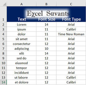
Let's assume that your dataset conforms to the following as shown in the image below:
Let's assume that your dataset conforms to the following as shown in the image below:
- Header in row 1
- Data to be conditionally formatted with custom font sizes is in cells A2:A100
- Font size specifications are in cells B2:B100
- To take it a step further, cells C2:C100 will specify the Font type to be used in the corresponding cells in column 'A'.
Next, insert the following into a new Module in Excel's VBA editor and then run the macro to apply the formatting:
Dim FontSize As Integer
Dim i As Integer
Dim FontName as String
'Counter is 'i'
For i = 2 To 100
'Sets Font Size
FontSize = Range("B" & i).Value
'Sets Font type
FontName = Range("C" & i).Value
'Conditionally Formats Data
Range("A" & i).Font.Name = FontName
Range("A" & i).Font.Size = FontSize
Next i
End Sub
Permanently associating workbook files with preferred version of Excel
09/29/2021

I run Windows 10 on a 64-bit operating system and want to upgrade from Excel 2010 to Excel 2019. However I don't want this change impacting my regular use of other Office 2010 applications like Outlook 2010, Word 2010 and PowerPoint 2010. The Office 2010 interface is so much simpler and cleaner and results in me being productive. There is no option when installing Office 2019 to unbundle other Office applications to only install Excel 2019. When trying to run both the 2019 and 2010 versions of Office, all my Office files only associate with whatever version of Office was last installed or "repaired". For example, after I have "repaired" Office 2010 to re-associate my Word and PowerPoint to open with Office 2010, if I try to right click on an Excel file and select always open with Excel 2019, it still opens with Excel 2010. Is there a way to re-associate all Excel file types to Excel 2019 without impacting my file associations for other Office applications?
You've identified a frustrating shortcoming with Microsoft Office in that the last version of Office installed or repaired will determine all Office file associations. As you've experienced, even if you right click on an Office file and choose "Open With..", navigate to the file path for the desired Office application and then check the box to 'Always use this app to open this file type' the file will still open using the version of Office last installed or repaired. There is however a simple workaround for this shortcoming.
After Excel 2019 has been installed on your computer, "repair" Office 2010 by selecting:
PC Settings>Apps>Microsoft Office Professional Plus 2010>Modify>Repair
This will re-associate all Office file types back to Office 2010.
Next navigate to the Office 2010 program folder. The file path will most likely be:
C:\Program Files\Microsoft Office\Office14
If however you have a 32-bit version of Office 2010 installed on your 64-bit machine then the Office 2010 file path will likely be:
C:\Program Files (x86)\Microsoft Office\Office14
Next locate the EXCEL.exe file in this Office 2010 program folder and rename that file to 'EXCEL2010'. This causes all file types associated with Excel 2010 which had previously been directed to the Office 2010 EXCEL.exe file path to lose that association.
Now right click on any .XLSX file and select 'choose another app' to open the file. Scroll to the bottom of the dialog box until you encounter the option to 'Look for another App on this PC'. Select this option and navigate to the file path for Office 2019 (likely either C:\Program Files (x86)\Microsoft Office\root\Office16 or C:\Program Files\Microsoft Office\root\Office16). Check the box to 'Always use this app to open this file type'. Repeat these steps to associate other Excel file types such as .CSV, .XLS, and .XLSM to Excel 2019.
Finally, navigate back to the Office 2010 program folder and rename the program file EXCEL2010 back to EXCEL.
All Excel file types will now by default be opened with Excel 2019 while all other Office files types such as .PPT, .DOCX .MSG will be opened with the appropriate Office 2010 application.
Solving for a lease payment in Excel
09/01/2021

Is there a formula in Excel to solve for a maximum lease payment when you know the total present value of future lease payments, the interest rate, and the number of periods?
Given the present value of a loan, the interest rate and the number of periods you can use Excel's PMT() function to solve for the lease payment. For example, if the present value of the loan is $5,300, the number of periods is 36 months and the annual interest rate is 8% then the formula to solve for the payment would be:
=PMT(8%/12,36,-5300,0) which is $166.
=PMT(8%/12,36,-5300,0) which is $166.
PC to Mac Excel file compatibility
06/22/2020

I’m a PC user and created a macro enabled file in Excel 2010 and saved it in the XLSM file format. When attempting to share the file with a Macintosh user who has Excel for Mac version 16.38 (20061401), the Mac user encounters this error message: “This workbook contains content which isn’t supported in this version of Excel. To view the unsupported content in the file, you can open the workbook as read-only”. Can you identify the PC to Mac compatibility issues within the file?
The most profound differences between the Windows version of Excel as compared to the Mac version lie in the handling of Visual Basic programming and ActiveX controls. The Windows Excel file in question contains ActiveX control buttons linked to macros. ActiveX controls will not work on Excel for Mac which is one of the root causes of the file incompatibility issues. There is a widely circulated rumor that this is because Apple banned ActiveX from the MacOS. In fact, it’s because ActiveX is a Microsoft software framework which the company chose not to extend to other platforms like MacOS. Since Microsoft dropped ActiveX support in 2012 (in conjunction with the release of Windows 8) it is unlikely that future software updates to Excel for Mac will include a fix for ActiveX operating system incompatibility between PCs and Macs. Normally the fix for this ActiveX issue would be to replace all ActiveX control buttons with Form control buttons. However, this file's ActiveX controls are directly linked to macros. To further complicate matters Form controls which contain VBA (i.e. are linked to macros) are also incompatible with the Mac version of Excel. In this case, I’d advise replacing all ActiveX controls with keyboard shortcuts to call the various macros. So instead of calling the macro by clicking an ActiveX button, the Mac Excel user would call the macro through keyboard shortcuts which you specify.
Unlike ActiveX which is a blatant incompatibility issue, visual basic code incompatibility between the Windows and Mac versions of Excel is more nuanced. Visual basic code written in Windows can call shared object libraries using DLL (dynamic-link library). These are objects in a library which contain code and data that can be used by more than one program at the same time. For example the workbook in question uses the shared object “ThisWorkbook.RefreshAll” to refresh all Pivot tables in the workbook. Unfortunately, the Mac version of Excel does not have the same extensive object library as the Windows version. And I have been unable to locate a resource which lists what VBA objects included in the Windows version of Excel are missing from the Mac version of Excel. Due to the severe limitations of Excel for Mac, I do not own a Mac and am therefore unable to user test your file on Excel for Mac. Consequently “ThisWorkbook.RefreshAll” may be a recognized object on the Mac version of Excel or it may not be. If it is not a recognized object then an error like the one identified in your question may result.
Microsoft’s offical response to this discrepancy in object libraries between the two platforms is that, “If you are authoring Macros for Office for Mac, you can use most of the same objects that are available in VBA for Office”. (https://docs.microsoft.com/en-us/office/vba/api/overview/office-mac). This statement seems purposely vague as the literal meaning of “most" is ‘more than half’. Said another way, the Mac version of Excel has an object library deficit of less than 50% as compared to the Windows version of Excel.
To address this issue of uncertainty over object inclusion in Excel for Mac, try breaking up your condensed code into groups of other similar objects. For example instead of using “ThisWorkbook.RefreshAll” to refresh all Pivot tables within the workbook, it's possible to combine multiple expressions of ActiveSheet.PivotTables("PivotTable1").PivotCache.Refresh with each expression specifying the sheet name and PivotTable number to refresh. Since this solution becomes too cumbersome and inefficient when there is complex VBA code, some Mac users choose to solve the incompatibility issue by running the Windows version of Excel on a virtual machine installed on the Mac operating system.
Excel 2010 protected workbook forgot password
10/23/2019

How do I open up a password protected Excel 2010 workbook if I can’t recall the password?
Before addressing your question it’s germane to understand the types of password protection options available in Excel 2010 and above. Password protection can be implemented at any or all of the following levels in Excel:
Worksheet-level:
A locked worksheet controls how users are able to interact with the worksheet. For example, worksheet protection can limit rows and columns from being added or deleted. Protection can also be extended to cells, ranges, formulas, and ActiveX or Form controls. Below are two approaches to unlocking the worksheet without the password:
WinZip Unlock Method:
In order to unlock a worksheet in the absence of the password, first rename the extension of the file from *.xlsx to *.zip. Then, using file compression software such as WinZip, open this .zip file. In the directory of folders, locate the “xl” folder and then the “worksheets” folder. Within the “worksheets” folder, select the locked worksheet(s) such as “sheet1.xml”. Next open this .xml file in the Notepad application. Search for the line of code that begins with “<sheetProtection algorithmName=”SHA-512″ hashValue=“ and then delete this entire line of code. Save the changes to this .xml file in the “worksheets” folder. Finally rename the extension of the overarching file from *.zip back to *.xlsx. The worksheet(s) will then be unprotected. Worksheets can also be unlocked via a macro using a combination of the visual basic arguments “ActiveSheet.Unprotect Chr” and “ActiveSheet.ProtectContents=FALSE”
Visual Basic Code Method
If the workbook's Visual Basic project has not been locked for viewing and you just want to unlock the worksheet and don't need to know the original password then the following VBA code should do the trick.
Sub CrackPass()
Const a = 65, b = 66, c = 32, d = 126
Dim i#, j#, k#, l#, m#, n#, o#, p#, q#, r#, s#, t#
With ActiveSheet
If .ProtectContents Then
On Error Resume Next
For i = a To b
For j = a To b
For k = a To b
For l = a To b
For m = a To b
For n = a To b
For o = a To b
For p = a To b
For q = a To b
For r = a To b
For s = a To b
For t = c To d
.Unprotect Chr(i) & Chr(j) & Chr(k) & Chr(l) & Chr(m) & _
Chr(n) & Chr(o) & Chr(p) & Chr(q) & Chr(r) & Chr(s) & Chr(t)
Next t
Next s
Next r
Next q
Next p
Next o
Next n
Next m
Next l
Next k
Next j
Next i
MsgBox "Workbook has been sucessfully unlocked"
End If
End With
End Sub
4. Press F5 or click the Run button on the toolbar to run the macro and wait for the worksheet to unlock.
Workbook structure-level:
Locking the workbook structure prevents users without the password from viewing hidden worksheets, adding, moving, deleting, renaming or hiding worksheets. The visual basic code below can be used to unlock the workbook structure without a password:
ActiveWorkbook.Unprotect “YourPassword”, True, True
Excel file-level:
Locking the file structure encrypts the Excel file and prevents the opening of the file without the password. It is not possible to unlock a secured Excel file without the password. Microsoft utilizes an Advanced Encryption Standard (AES) and a 128-bit key so the only way to break the password is by using third-party password hacking software. Keep in mind that these software programs may harbor malicious algorithms and present a serious security risk.
- Worksheet level
- Workbook structure level
- File level
- Visual Basic editor
Worksheet-level:
A locked worksheet controls how users are able to interact with the worksheet. For example, worksheet protection can limit rows and columns from being added or deleted. Protection can also be extended to cells, ranges, formulas, and ActiveX or Form controls. Below are two approaches to unlocking the worksheet without the password:
WinZip Unlock Method:
In order to unlock a worksheet in the absence of the password, first rename the extension of the file from *.xlsx to *.zip. Then, using file compression software such as WinZip, open this .zip file. In the directory of folders, locate the “xl” folder and then the “worksheets” folder. Within the “worksheets” folder, select the locked worksheet(s) such as “sheet1.xml”. Next open this .xml file in the Notepad application. Search for the line of code that begins with “<sheetProtection algorithmName=”SHA-512″ hashValue=“ and then delete this entire line of code. Save the changes to this .xml file in the “worksheets” folder. Finally rename the extension of the overarching file from *.zip back to *.xlsx. The worksheet(s) will then be unprotected. Worksheets can also be unlocked via a macro using a combination of the visual basic arguments “ActiveSheet.Unprotect Chr” and “ActiveSheet.ProtectContents=FALSE”
Visual Basic Code Method
If the workbook's Visual Basic project has not been locked for viewing and you just want to unlock the worksheet and don't need to know the original password then the following VBA code should do the trick.
- Press Alt + F11 to open the Visual Basic Editor.
- Right-click the workbook name on the left pane (Project-VBAProject pane) and select Insert > Module from the context menu.
- In the window that appears, paste in the following code:
Sub CrackPass()
Const a = 65, b = 66, c = 32, d = 126
Dim i#, j#, k#, l#, m#, n#, o#, p#, q#, r#, s#, t#
With ActiveSheet
If .ProtectContents Then
On Error Resume Next
For i = a To b
For j = a To b
For k = a To b
For l = a To b
For m = a To b
For n = a To b
For o = a To b
For p = a To b
For q = a To b
For r = a To b
For s = a To b
For t = c To d
.Unprotect Chr(i) & Chr(j) & Chr(k) & Chr(l) & Chr(m) & _
Chr(n) & Chr(o) & Chr(p) & Chr(q) & Chr(r) & Chr(s) & Chr(t)
Next t
Next s
Next r
Next q
Next p
Next o
Next n
Next m
Next l
Next k
Next j
Next i
MsgBox "Workbook has been sucessfully unlocked"
End If
End With
End Sub
4. Press F5 or click the Run button on the toolbar to run the macro and wait for the worksheet to unlock.
Workbook structure-level:
Locking the workbook structure prevents users without the password from viewing hidden worksheets, adding, moving, deleting, renaming or hiding worksheets. The visual basic code below can be used to unlock the workbook structure without a password:
ActiveWorkbook.Unprotect “YourPassword”, True, True
Excel file-level:
Locking the file structure encrypts the Excel file and prevents the opening of the file without the password. It is not possible to unlock a secured Excel file without the password. Microsoft utilizes an Advanced Encryption Standard (AES) and a 128-bit key so the only way to break the password is by using third-party password hacking software. Keep in mind that these software programs may harbor malicious algorithms and present a serious security risk.
External data Import errors
09/31/2019

Why can’t I import data from certain websites using Microsoft Excel?
Excel versions 1997 - 2010 rely on a rudimentary native browser for external data queries which is unable to handle modern website features like Adobe flash and ad trackers. As a result, you’ll often encounter a litany of script errors when attempting to set up a link to a live external data source using this built-in web browser. While you may be able to click through these script errors and proceed with establishing the external data link, there will be times when an external data query link cannot be established due to these script errors and the Excel program may crash.
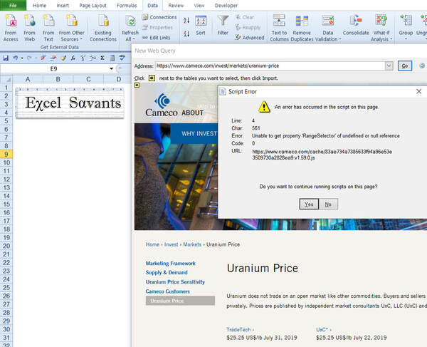
There is however an elegant solution to this problem. Beginning with the Excel 2016 build, Microsoft launched an enhanced data query tool called “Power Query” which is able to process data pulls from websites which earlier versions of Excel could not handle. If you are using Excel 2003 or Excel 2010, you can download the free Power Query Add-In from the Microsoft office support website.
Conditional formatting to highlight cells based on data in another cell
08/19/2019

Can I use conditional formatting in Excel 2010 to highlight cells according to a date found in another column?
Conditionally highlighting cells in one column based data in another column can be easily accomplished using Excel’s Conditional Formatting functionality.
For example, assume you have a list of event dates in column ‘A’ and you want to highlight the corresponding event descriptions in column ‘B’ if the date in column ‘A’ occurs before 11/02/2019.
Since the conditional formatting formula requires that dates used directly in the formula be in the Excel “serial” date format (Excel stores dates as sequential serial numbers, with January 1, 1900 being serial number 1, because it’s more efficient for use in date calculations), you’ll want to convert 11/02/2019 to this format. To determine the Excel serial date of 11/02/2019, input this value into any cell in your worksheet and then change the format of that cell from ‘date’ to ‘number’. The Excel serial number 43771 will be displayed in this cell because it is 43770 days after January 1, 1900 which is serial number 1.
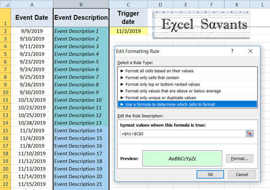
To create the conditional formatting formula, first highlight column ‘B’. Then navigate to the Excel Ribbon, select Conditional Formatting then “New Rule” then “Use a formula to determine which cells to format". In the formula box input =$A1<43771. Alternatively if the date 11/02/2019 is located in cell C2, the formula can be written as =$A1<$C$2. Next choose how you’d like to format cells that meet this criteria for example by filling the cells with a light green fill and displaying text in an italic font style.
The event descriptions in column ‘B’ with corresponding dates in column ‘A’ which occur before 11/02/2019 will now be formatted with a light green fill and an italic font style.
The event descriptions in column ‘B’ with corresponding dates in column ‘A’ which occur before 11/02/2019 will now be formatted with a light green fill and an italic font style.
How can you hide a row within Excel using a formula based on a condition?
08/11/2019
There is no native Excel formula which allows you to conditionally hide an entire row based on user-defined criteria. You can however create a simple macro which would leverage the VBA command “EntireRow.Hidden” to accomplish this.
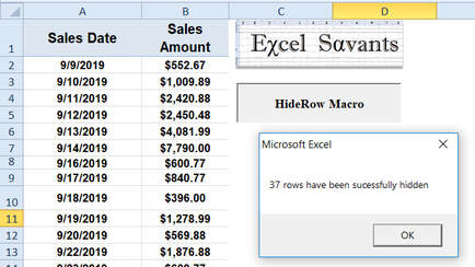
For example, let’s assume you have a worksheet with daily sales figures in column B (column number 2) for a sole proprietorship brick and mortar retail business for the last 12 months and there’s one header row followed by 365 rows of data representing each day of the last year (for a total of 366 rows). However, while this single employee business is generally open 7 days a week, it is closed on various holidays and when the owner is on vacation. The sales data is directly exported from the business Point of Sale system which does not account for whether the business is open on any given day. Instead of manually hiding the rows of data corresponding to when the business is closed, you want Excel to automatically perform this task. You can insert an ‘Active X’ command button into the worksheet which could launch the following macro I have written for you at the click of a button. When executed, the macro examines each of the 365 rows of sales data in column B of the worksheet and then hides any row where the sales for that day is less than $.01. When the macro has completed its tasks, a dialog box appears detailing how many rows have been hidden. I have included a example file below available for download as well as the VBA code for this macro.
For example, let’s assume you have a worksheet with daily sales figures in column B (column number 2) for a sole proprietorship brick and mortar retail business for the last 12 months and there’s one header row followed by 365 rows of data representing each day of the last year (for a total of 366 rows). However, while this single employee business is generally open 7 days a week, it is closed on various holidays and when the owner is on vacation. The sales data is directly exported from the business Point of Sale system which does not account for whether the business is open on any given day. Instead of manually hiding the rows of data corresponding to when the business is closed, you want Excel to automatically perform this task. You can insert an ‘Active X’ command button into the worksheet which could launch the following macro I have written for you at the click of a button. When executed, the macro examines each of the 365 rows of sales data in column B of the worksheet and then hides any row where the sales for that day is less than $.01. When the macro has completed its tasks, a dialog box appears detailing how many rows have been hidden. I have included a example file below available for download as well as the VBA code for this macro.
| Excel Savants LLC Example File-Hide Row based on condition |
Sub HideRow()
Dim Hidecount As Integer
StartRow = 2
EndRow = 366
ColumnNum = 2
Hidecount = 0
For RowCnt = StartRow To EndRow
If Cells(RowCnt, ColumnNum).Value < .01 Then
Hidecount = Hidecount + 1
Cells(RowCnt, ColumnNum).EntireRow.Hidden = True
Else
Cells(RowCnt, ColumnNum).EntireRow.Hidden = False
End If
Next RowCnt
MsgBox Hidecount & " rows have been sucessfully hidden"
End Sub
What is the significance of the number of columns at 16,384 in Excel 2016? Why didn’t Microsoft go further, up to columun`ZZZ` (17,576) instead of stopping at `XFD` (16,384)?
07/25/2019
I would speculate that the number of columns at 16,384 was likely chosen to optimize allocation of computer memory resources. Excel is performing ongoing checks to see if its cell limit has been exceeded. Note that 16,384 = 2^14 which represents a 3-letter "bit" in computing terms. However 2^15 would enter 4-letter bit territory which requires significantly more memory allocation to process. By limiting the bounds of the columns to 2^14, Excel is maximizing computer memory resources.
How can I split a single Excel column of data into two columns by using RPA automation anywhere in an Excel sheet?
07/08/2019
It is not apparent what sort of rule-driven robotic process automation (RPA) you are envisioning or what you are specifically referring to by "splitting" a column of Excel data. If you have grouped data that needs to be divided into multiple columns, a visual basic macro could deftly perform this task. The macro would use the "Selection.Columns.Ungroup" command (and/ or the "EntireColumn.Insert" command depending on the task you are trying to accomplish). This macro could be set to run either at the click of a button or when some other user-specified event occurs.
If you'd like the code for creating a macro to split columns, then please submit a new Answer Forum request and include an explanation of what you mean by splitting columns of data and what, in your mind, constitutes RPA automation.
If you'd like the code for creating a macro to split columns, then please submit a new Answer Forum request and include an explanation of what you mean by splitting columns of data and what, in your mind, constitutes RPA automation.
Excel - How do I get a cell to return a value for background colors of a cell?
07/02/2019
The optimal way to return the background color in Excel is to:
1) Create a user-defined function (UDF) in Excel’s Visual Basic editor. In the example below, I have named the UDF “Get_Cell_Color”.
To create this UDF, insert a new module into Excel’s Visual Basic editor and then input this code:
Function Get_Cell_Color(FCell As Range) As String
'Returns the Cell color
Dim xColor As String
xColor = CStr(FCell.Interior.Color)
xColor = Right("000000" & Hex(xColor), 6)
Get_Cell_Color = Right(xColor, 2) & Mid(xColor, 3, 2) & Left(xColor, 2)
End Function
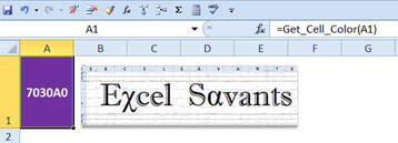
2) Call this UDF for the cell in which you want to evaluate the background color just as you would call any other Excel formula. For example, the formula to evaluate the background color of cell “A1” would be: "=Get_Cell_Color(A1)". If cell A1 is filled with Excel’s “standard” purple color then the UDF formula would return a cell fill color code value of “7030A0”.
1) Create a user-defined function (UDF) in Excel’s Visual Basic editor. In the example below, I have named the UDF “Get_Cell_Color”.
To create this UDF, insert a new module into Excel’s Visual Basic editor and then input this code:
Function Get_Cell_Color(FCell As Range) As String
'Returns the Cell color
Dim xColor As String
xColor = CStr(FCell.Interior.Color)
xColor = Right("000000" & Hex(xColor), 6)
Get_Cell_Color = Right(xColor, 2) & Mid(xColor, 3, 2) & Left(xColor, 2)
End Function
2) Call this UDF for the cell in which you want to evaluate the background color just as you would call any other Excel formula. For example, the formula to evaluate the background color of cell “A1” would be: "=Get_Cell_Color(A1)". If cell A1 is filled with Excel’s “standard” purple color then the UDF formula would return a cell fill color code value of “7030A0”.
Note that this example UDF is by default considered to have a “public” scope by Excel meaning that it is available for all sheets in the Workbook as well as all the procedures (Sub and Function) across every module in the Workbook. However, the UDF is not available for use in other Excel workbooks unless you:
a) Create an “Add-in” and install it on your Excel application.
and/or
b) Save the UDF in the Personal Macro Workbook (which is a hidden system file that opens with the Excel application).
If you are interested in learning more about creating an “Add-in” and/or the Personal Macro Workbook then please submit a new Answer Forum request.
What’s the most useful MS Excel trick you know?
05/26/2019
An often underappreciated capability of Excel is that it can be programmed to communicate with other Microsoft applications and even Adobe PDF viewer using Object Linking and Embedding (OLE) Automation. For example, you could create Visual Basic macros in Excel which at the click of a button would allow you to export an Excel chart into a PowerPoint slide or export an Excel form into a PDF or Microsoft Word file.
Is it possible to link an Excel planner to a Google calendar?
05/23/2019
You can link an event in your Excel based calendar to your Google Calendar by inserting a hyperlink in Excel to the unique URL for the corresponding event in your Google Calendar. However it is not possible to dynamically "link" an entire Excel based calendar to Google Calendar so that event updates in Excel will automatically be reflected in your Google Calendar.
You can however create a simple Excel based process to export new calendar events to a CSV file which you can then manually upload to Google Calendar:
1) Insert a worksheet into your Excel planner with row headers which exactly match the Google Calendar fields listed here: https://support.google.com/calendar/answer/37118?hl=en.
2) Have the fields in the worksheet reference the relevant event fields from elsewhere in your Excel planner. For example if the new worksheet is ‘Sheet 2’ and the event data source is on ‘Sheet 1’ then map the cells in ‘Sheet 2’ to the corresponding cells in ‘Sheet 1’
3) Insert an ‘Active X’ button on the new worksheet which links to a macro which first saves this worksheet as a separate CSV file to your desktop and then opens the following hyperlink: https://calendar.google.com/calendar/r/settings/export
4) Execute the macro by clicking the ‘Active X’ button. Once the Google Calendar import dialog opens, select the new CSV file on your desktop and import that file to your Google Calendar.
What function should I input in Excel to implement this command, “If a cell in one sheet contains one word, then print a range of cells from another sheet right under it”?
04/13/2019
There is no built-in Excel function which would accomplish this. However, you can insert an ‘Active X’ command button and a simple macro into your Excel workbook which, at the click of a button, would search for your keyword in 'Sheet 1' and then if the keyword is found, a command to print a range of cells in 'Sheet 2' would execute. In the VBA code below, the word being searched in 'Sheet 1' is “Keyword” and the print range in 'Sheet 2' is cells “A2:G20”. If the word you are searching for is expected to change over time, then I’d suggest editing the macro to have it either prompt you for the search word upon execution or have the macro reference a static cell in 'Sheet 1' where you can input your search word.
Sub Print_from_Keyword()
Dim FindWord As String
Dim Found As Range
FindWord = "Keyword"
Set Found = Sheets("Sheet1").Cells.Find(What:=FindWord, _
LookIn:=xlValues, _
LookAt:=xlPart, _
SearchOrder:=xlByRows, _
SearchDirection:=xlNext, _
MatchCase:=False)
If Not Found Is Nothing Then
Sheet("Sheet2").Select
Range("A2:G20").Select
ActiveSheet.PageSetup.PrintArea = "A2:G20"
ActiveWindow.SelectedSheets.PrintOut From:=1, To:=1, Copies:=1, Collate _:=True
Else
MsgBox "The Keyword was not found."
End If
End Sub
How can I move data from one sheet onto another at a certain time?
03/10/2019
This is an excellent question. I'd advise creating/ recording a simple macro which copies data from Sheet 1 to Sheet 2. Next you'll want to edit this macro and insert the "Application.OnTime" VBA application object. This will allow you to schedule the macro to automatically run at your specified time and date in the future.
If this is a procedure you will be performing regularly, I'd suggest having the macro prompt you for variable inputs such as the date and time you want to run the module next. Note that the Excel workbook with the embedded macro must be open at the scheduled execution time in order for the macro to run.
For details on the syntax of this object and how to use it, I'd suggest visiting: https://docs.microsoft.com/en-us/office/vba/api/excel.application.ontime
What is the formula in Excel for a Zigzag indicator?
01/10/2019
The so-called Zigzag oscillator is the output of several variables and depends on what dataset you are using and your percentage of price movement tolerance. There is no one universal formula for this. I'd suggest creating a simple model to determine the support and resistance areas in your asset price dataset. Once you have done that and if you have specific questions feel free to submit a new Answer Forum request and I will respond.
What is the benefit of using Select Case over If-Then in Excel VBA?
11/19/2018
When coding in VBA, SELECT CASE and IF THEN provide the same result. However, SELECT CASE is a better choice if you have numerous Cases/ Conditions. It is cleaner and easier code to read as indented CASE statements as opposed to a litany of IF-THEN-ELSE IF statements. Alternatively, if you have a very large number of Conditions/ Cases, an ARRAY is a better coding choice.
|
Please consider supporting the Excel Savants Answer Forum by visiting our advertisers:
|